chronon

Chronon is a data platform for serving for AI/ML applications.

Stars: 766

Visit

Chronon is a platform that simplifies and improves ML workflows by providing a central place to define features, ensuring point-in-time correctness for backfills, simplifying orchestration for batch and streaming pipelines, offering easy endpoints for feature fetching, and guaranteeing and measuring consistency. It offers benefits over other approaches by enabling the use of a broad set of data for training, handling large aggregations and other computationally intensive transformations, and abstracting away the infrastructure complexity of data plumbing.

README:

Chronon: A Data Platform for AI/ML

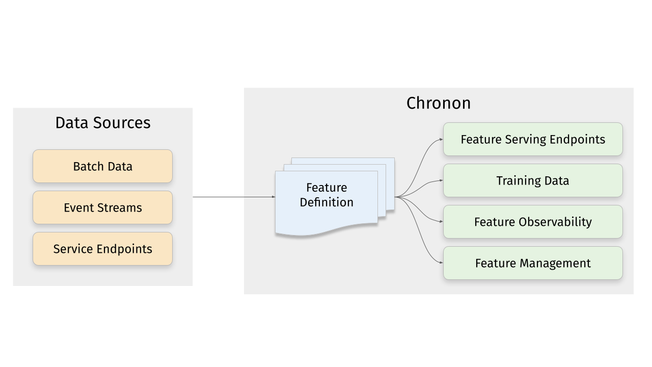
Chronon is a platform that abstracts away the complexity of data computation and serving for AI/ML applications. Users define features as transformation of raw data, then Chronon can perform batch and streaming computation, scalable backfills, low-latency serving, guaranteed correctness and consistency, as well as a host of observability and monitoring tools.

It allows you to utilize all of the data within your organization, from batch tables, event streams or services to power your AI/ML projects, without needing to worry about all the complex orchestration that this would usually entail.

More information about Chronon can be found at chronon.ai.

Platform Features

Online Serving

Chronon offers an API for realtime fetching which returns up-to-date values for your features. It supports:

Managed pipelines for batch and realtime feature computation and updates to the serving backend
Low latency serving of computed features
Scalable for high fanout feature sets

Backfills

ML practitioners often need historical views of feature values for model training and evaluation. Chronon's backfills are:

Scalable for large time windows
Resilient to highly skewed data
Point-in-time accurate such that consistency with online serving is guaranteed

Observability, monitoring and data quality

Chronon offers visibility into:

Data freshness - ensure that online values are being updated in realtime
Online/Offline consistency - ensure that backfill data for model training and evaluation is consistent with what is being observed in online serving

Complex transformations and windowed aggregations

Chronon supports a range of aggregation types. For a full list see the documentation here.

These aggregations can all be configured to be computed over arbitrary window sizes.

Quickstart

This section walks you through the steps to create a training dataset with Chronon, using a fabricated underlying raw dataset.

Includes:

Example implementation of the main API components for defining features - GroupBy and Join.
The workflow for authoring these entities.
The workflow for backfilling training data.
The workflows for uploading and serving this data.
The workflow for measuring consistency between backfilled training data and online inference data.

Does not include:

A deep dive on the various concepts and terminologies in Chronon. For that, please see the Introductory documentation.
Running streaming jobs.

Requirements

Docker

Setup

To get started with the Chronon, all you need to do is download the docker-compose.yml file and run it locally:

curl -o docker-compose.yml https://chronon.ai/docker-compose.yml
docker-compose up

Once you see some data printed with a only showing top 20 rows notice, you're ready to proceed with the tutorial.

Introduction

In this example, let's assume that we're a large online retailer, and we've detected a fraud vector based on users making purchases and later returning items. We want to train a model that will be called when the checkout flow commences and predicts whether this transaction is likely to result in a fraudulent return.

Raw data sources

Fabricated raw data is included in the data directory. It includes four tables:

Users - includes basic information about users such as account created date; modeled as a batch data source that updates daily
Purchases - a log of all purchases by users; modeled as a log table with a streaming (i.e. Kafka) event-bus counterpart
Returns - a log of all returns made by users; modeled as a log table with a streaming (i.e. Kafka) event-bus counterpart
Checkouts - a log of all checkout events; this is the event that drives our model predictions

Start a shell session in the Docker container

In a new terminal window, run:

docker-compose exec main bash

This will open a shell within the chronon docker container.

Chronon Development

Now that the setup steps are complete, we can start creating and testing various Chronon objects to define transformation and aggregations, and generate data.

Step 1 - Define some features

Let's start with three feature sets, built on top of our raw input sources.

Note: These python definitions are already in your chronon image. There's nothing for you to run until Step 3 - Backfilling Data when you'll run computation for these definitions.

Feature set 1: Purchases data features

We can aggregate the purchases log data to the user level, to give us a view into this user's previous activity on our platform. Specifically, we can compute SUMs COUNTs and AVERAGEs of their previous purchase amounts over various windows.

Because this feature is built upon a source that includes both a table and a topic, its features can be computed in both batch and streaming.

source = Source(
    events=EventSource(
        table="data.purchases", # This points to the log table with historical purchase events
        topic=None, # Streaming is not currently part of quickstart, but this would be where you define the topic for realtime events
        query=Query(
            selects=select("user_id","purchase_price"), # Select the fields we care about
            time_column="ts") # The event time
    ))

window_sizes = [Window(length=day, timeUnit=TimeUnit.DAYS) for day in [3, 14, 30]] # Define some window sizes to use below

v1 = GroupBy(
    sources=[source],
    keys=["user_id"], # We are aggregating by user
    aggregations=[Aggregation(
            input_column="purchase_price",
            operation=Operation.SUM,
            windows=window_sizes
        ), # The sum of purchases prices in various windows
        Aggregation(
            input_column="purchase_price",
            operation=Operation.COUNT,
            windows=window_sizes
        ), # The count of purchases in various windows
        Aggregation(
            input_column="purchase_price",
            operation=Operation.AVERAGE,
            windows=window_sizes
        ) # The average purchases by user in various windows
    ],
)

See the whole code file here: purchases GroupBy. This is also in your docker image. We'll be running computation for it and the other GroupBys in Step 3 - Backfilling Data.

Feature set 2: Returns data features

We perform a similar set of aggregations on returns data in the returns GroupBy. The code is not included here because it looks similar to the above example.

Feature set 3: User data features

Turning User data into features is a littler simpler, primarily because there are no aggregations to include. In this case, the primary key of the source data is the same as the primary key of the feature, so we're simply extracting column values rather than performing aggregations over rows:

source = Source(
    entities=EntitySource(
        snapshotTable="data.users", # This points to a table that contains daily snapshots of the entire product catalog
        query=Query(
            selects=select("user_id","account_created_ds","email_verified"), # Select the fields we care about
        )
    ))

v1 = GroupBy(
    sources=[source],
    keys=["user_id"], # Primary key is the same as the primary key for the source table
    aggregations=None # In this case, there are no aggregations or windows to define
)

Taken from the users GroupBy.

Step 2 - Join the features together

Next, we need the features that we previously defined backfilled in a single table for model training. This can be achieved using the Join API.

For our use case, it's very important that features are computed as of the correct timestamp. Because our model runs when the checkout flow begins, we'll want to be sure to use the corresponding timestamp in our backfill, such that features values for model training logically match what the model will see in online inference.

Join is the API that drives feature backfills for training data. It primarilly performs the following functions:

Combines many features together into a wide view (hence the name Join).
Defines the primary keys and timestamps for which feature backfills should be performed. Chronon can then guarantee that feature values are correct as of this timestamp.
Performs scalable backfills.

Here is what our join looks like:

source = Source(
    events=EventSource(
        table="data.checkouts", 
        query=Query(
            selects=select("user_id"), # The primary key used to join various GroupBys together
            time_column="ts",
            ) # The event time used to compute feature values as-of
    ))

v1 = Join(  
    left=source,
    right_parts=[JoinPart(group_by=group_by) for group_by in [purchases_v1, refunds_v1, users]] # Include the three GroupBys
)

Taken from the training_set Join.

The left side of the join is what defines the timestamps and primary keys for the backfill (notice that it is built on top of the checkout event, as dictated by our use case).

Note that this Join combines the above three GroupBys into one data definition. In the next step, we'll run the command to execute computation for this whole pipeline.

Step 3 - Backfilling Data

Once the join is defined, we compile it using this command:

compile.py --conf=joins/quickstart/training_set.py

This converts it into a thrift definition that we can submit to spark with the following command:

run.py --conf production/joins/quickstart/training_set.v1

The output of the backfill would contain the user_id and ts columns from the left source, as well as the 11 feature columns from the three GroupBys that we created.

Feature values would be computed for each user_id and ts on the left side, with guaranteed temporal accuracy. So, for example, if one of the rows on the left was for user_id = 123 and ts = 2023-10-01 10:11:23.195, then the purchase_price_avg_30d feature would be computed for that user with a precise 30 day window ending on that timestamp.

You can now query the backfilled data using the spark sql shell:

spark-sql

And then:

spark-sql> SELECT user_id, quickstart_returns_v1_refund_amt_sum_30d, quickstart_purchases_v1_purchase_price_sum_14d, quickstart_users_v1_email_verified from default.quickstart_training_set_v1 limit 100;

Note that this only selects a few columns. You can also run a select * from default.quickstart_training_set_v1 limit 100 to see all columns, however, note that the table is quite wide and the results might not be very readable on your screen.

To exit the sql shell you can run:

spark-sql> quit;

Online Flows

Now that we've created a join and backfilled data, the next step would be to train a model. That is not part of this tutorial, but assuming it was complete, the next step after that would be to productionize the model online. To do this, we need to be able to fetch feature vectors for model inference. That's what this next section covers.

Uploading data

In order to serve online flows, we first need the data uploaded to the online KV store. This is different than the backfill that we ran in the previous step in two ways:

The data is not a historic backfill, but rather the most up-to-date feature values for each primary key.
The datastore is a transactional KV store suitable for point lookups. We use MongoDB in the docker image, however you are free to integrate with a database of your choice.

Upload the purchases GroupBy:

run.py --mode upload --conf production/group_bys/quickstart/purchases.v1 --ds  2023-12-01

spark-submit --class ai.chronon.quickstart.online.Spark2MongoLoader --master local[*] /srv/onlineImpl/target/scala-2.12/mongo-online-impl-assembly-0.1.0-SNAPSHOT.jar default.quickstart_purchases_v1_upload mongodb://admin:admin@mongodb:27017/?authSource=admin

Upload the returns GroupBy:

run.py --mode upload --conf production/group_bys/quickstart/returns.v1 --ds  2023-12-01

spark-submit --class ai.chronon.quickstart.online.Spark2MongoLoader --master local[*] /srv/onlineImpl/target/scala-2.12/mongo-online-impl-assembly-0.1.0-SNAPSHOT.jar default.quickstart_returns_v1_upload mongodb://admin:admin@mongodb:27017/?authSource=admin

Upload Join Metadata

If we want to use the FetchJoin api rather than FetchGroupby, then we also need to upload the join metadata:

run.py --mode metadata-upload --conf production/joins/quickstart/training_set.v2

This makes it so that the online fetcher knows how to take a request for this join and break it up into individual GroupBy requests, returning the unified vector, similar to how the Join backfill produces the wide view table with all features.

Fetching Data

With the above entities defined, you can now easily fetch feature vectors with a simple API call.

Fetching a join:

run.py --mode fetch --type join --name quickstart/training_set.v2 -k '{"user_id":"5"}'

You can also fetch a single GroupBy (this would not require the Join metadata upload step performed earlier):

run.py --mode fetch --type group-by --name quickstart/purchases.v1 -k '{"user_id":"5"}'

For production, the Java client is usually embedded directly into services.

Map<String, String> keyMap = new HashMap<>();
keyMap.put("user_id", "123");
Fetcher.fetch_join(new Request("quickstart/training_set_v1", keyMap))

sample response

> '{"purchase_price_avg_3d":14.3241, "purchase_price_avg_14d":11.89352, ...}'

Note: This java code is not runnable in the docker env, it is just an illustrative example.

Log fetches and measure online/offline consistency

As discussed in the introductory sections of this README, one of Chronon's core guarantees is online/offline consistency. This means that the data that you use to train your model (offline) matches the data that the model sees for production inference (online).

A key element of this is temporal accuracy. This can be phrased as: when backfilling features, the value that is produced for any given timestamp provided by the left side of the join should be the same as what would have been returned online if that feature was fetched at that particular timestamp.

Chronon not only guarantees this temporal accuracy, but also offers a way to measure it.

The measurement pipeline starts with the logs of the online fetch requests. These logs include the primary keys and timestamp of the request, along with the fetched feature values. Chronon then passes the keys and timestamps to a Join backfill as the left side, asking the compute engine to backfill the feature values. It then compares the backfilled values to actual fetched values to measure consistency.

Step 1: log fetches

First, make sure you've ran a few fetch requests. Run:

run.py --mode fetch --type join --name quickstart/training_set.v2 -k '{"user_id":"5"}'

A few times to generate some fetches.

With that complete, you can run this to create a usable log table (these commands produce a logging hive table with the correct schema):

spark-submit --class ai.chronon.quickstart.online.MongoLoggingDumper --master local[*] /srv/onlineImpl/target/scala-2.12/mongo-online-impl-assembly-0.1.0-SNAPSHOT.jar default.chronon_log_table mongodb://admin:admin@mongodb:27017/?authSource=admin
compile.py --conf group_bys/quickstart/schema.py
run.py --mode backfill --conf production/group_bys/quickstart/schema.v1
run.py --mode log-flattener --conf production/joins/quickstart/training_set.v2 --log-table default.chronon_log_table --schema-table default.quickstart_schema_v1

This creates a default.quickstart_training_set_v2_logged table that contains the results of each of the fetch requests that you previously made, along with the timestamp at which you made them and the user that you requested.

Note: Once you run the above command, it will create and "close" the log partitions, meaning that if you make additional fetches on the same day (UTC time) it will not append. If you want to go back and generate more requests for online/offline consistency, you can drop the table (run DROP TABLE default.quickstart_training_set_v2_logged in a spark-sql shell) before rerunning the above command.

Now you can compute consistency metrics with this command:

run.py --mode consistency-metrics-compute --conf production/joins/quickstart/training_set.v2

This job will take the primary key(s) and timestamps from the log table (default.quickstart_training_set_v2_logged in this case), and uses those to create and run a join backfill. It then compares the backfilled results to the actual logged values that were fetched online

It produces two output tables:

default.quickstart_training_set_v2_consistency: A human readable table that you can query to see the results of the consistency checks.
1. You can enter a sql shell by running spark-sql from your docker bash sesion, then query the table.
2. Note that it has many columns (multiple metrics per feature), so you might want to run a DESC default.quickstart_training_set_v2_consistency first, then select a few columns that you care about to query.
default.quickstart_training_set_v2_consistency_upload: A list of KV bytes that is uploaded to the online KV store, that can be used to power online data quality monitoring flows. Not meant to be human readable.

Conclusion

Using chronon for your feature engineering work simplifies and improves your ML Workflow in a number of ways:

You can define features in one place, and use those definitions both for training data backfills and for online serving.
Backfills are automatically point-in-time correct, which avoids label leakage and inconsistencies between training data and online inference.
Orchestration for batch and streaming pipelines to keep features up to date is made simple.
Chronon exposes easy endpoints for feature fetching.
Consistency is guaranteed and measurable.

For a more detailed view into the benefits of using Chronon, see Benefits of Chronon documentation.

Benefits of Chronon over other approaches

Chronon offers the most value to AI/ML practitioners who are trying to build "online" models that are serving requests in real-time as opposed to batch workflows.

Without Chronon, engineers working on these projects need to figure out how to get data to their models for training/eval as well as production inference. As the complexity of data going into these models increases (multiple sources, complex transformation such as windowed aggregations, etc), so does the infrastructure challenge of supporting this data plumbing.

Generally, we observed ML practitioners taking one of two approaches:

The log-and-wait approach

With this approach, users start with the data that is available in the online serving environment from which the model inference will run. Log relevant features to the data warehouse. Once enough data has accumulated, train the model on the logs, and serve with the same data.

Pros:

Features used to train the model are guaranteed to be available at serving time
The model can access service call features
The model can access data from the the request context

Cons:

It might take a long to accumulate enough data to train the model
Performing windowed aggregations is not always possible (running large range queries against production databases doesn't scale, same for event streams)
Cannot utilize the wealth of data already in the data warehouse
Maintaining data transformation logic in the application layer is messy

The replicate offline-online approach

With this approach, users train the model with data from the data warehouse, then figure out ways to replicate those features in the online environment.

Pros:

You can use a broad set of data for training
The data warehouse is well suited for large aggregations and other computationally intensive transformation

Cons:

Often very error prone, resulting in inconsistent data between training and serving
Requires maintaining a lot of complicated infrastructure to even get started with this approach,
Serving features with realtime updates gets even more complicated, especially with large windowed aggregations
Unlikely to scale well to many models

The Chronon approach

With Chronon you can use any data available in your organization, including everything in the data warehouse, any streaming source, service calls, etc, with guaranteed consistency between online and offline environments. It abstracts away the infrastructure complexity of orchestrating and maintining this data plumbing, so that users can simply define features in a simple API, and trust Chronon to handle the rest.

Contributing

We welcome contributions to the Chronon project! Please read CONTRIBUTING for details.

Support

Use the GitHub issue tracker for reporting bugs or feature requests. Join our community Slack workspace for discussions, tips, and support.

For Tasks:

Click tags to check more tools for each tasks

define features backfill training data serve features measure consistency

For Jobs:

data engineer machine learning engineer data scientist software engineer developer

Alternative AI tools for chronon

Similar Open Source Tools

chronon

github

: 766

PromptAgent

PromptAgent is a repository for a novel automatic prompt optimization method that crafts expert-level prompts using language models. It provides a principled framework for prompt optimization by unifying prompt sampling and rewarding using MCTS algorithm. The tool supports different models like openai, palm, and huggingface models. Users can run PromptAgent to optimize prompts for specific tasks by strategically sampling model errors, generating error feedbacks, simulating future rewards, and searching for high-reward paths leading to expert prompts.

github

: 150

rag-experiment-accelerator

The RAG Experiment Accelerator is a versatile tool that helps you conduct experiments and evaluations using Azure AI Search and RAG pattern. It offers a rich set of features, including experiment setup, integration with Azure AI Search, Azure Machine Learning, MLFlow, and Azure OpenAI, multiple document chunking strategies, query generation, multiple search types, sub-querying, re-ranking, metrics and evaluation, report generation, and multi-lingual support. The tool is designed to make it easier and faster to run experiments and evaluations of search queries and quality of response from OpenAI, and is useful for researchers, data scientists, and developers who want to test the performance of different search and OpenAI related hyperparameters, compare the effectiveness of various search strategies, fine-tune and optimize parameters, find the best combination of hyperparameters, and generate detailed reports and visualizations from experiment results.

github

: 242

AIlice

AIlice is a fully autonomous, general-purpose AI agent that aims to create a standalone artificial intelligence assistant, similar to JARVIS, based on the open-source LLM. AIlice achieves this goal by building a "text computer" that uses a Large Language Model (LLM) as its core processor. Currently, AIlice demonstrates proficiency in a range of tasks, including thematic research, coding, system management, literature reviews, and complex hybrid tasks that go beyond these basic capabilities. AIlice has reached near-perfect performance in everyday tasks using GPT-4 and is making strides towards practical application with the latest open-source models. We will ultimately achieve self-evolution of AI agents. That is, AI agents will autonomously build their own feature expansions and new types of agents, unleashing LLM's knowledge and reasoning capabilities into the real world seamlessly.

github

: 1.1k

pgai

pgai simplifies the process of building search and Retrieval Augmented Generation (RAG) AI applications with PostgreSQL. It brings embedding and generation AI models closer to the database, allowing users to create embeddings, retrieve LLM chat completions, reason over data for classification, summarization, and data enrichment directly from within PostgreSQL in a SQL query. The tool requires an OpenAI API key and a PostgreSQL client to enable AI functionality in the database. Users can install pgai from source, run it in a pre-built Docker container, or enable it in a Timescale Cloud service. The tool provides functions to handle API keys using psql or Python, and offers various AI functionalities like tokenizing, detokenizing, embedding, chat completion, and content moderation.

github

: 5.7k

lumigator

Lumigator is an open-source platform developed by Mozilla.ai to help users select the most suitable language model for their specific needs. It supports the evaluation of summarization tasks using sequence-to-sequence models such as BART and BERT, as well as causal models like GPT and Mistral. The platform aims to make model selection transparent, efficient, and empowering by providing a framework for comparing LLMs using task-specific metrics to evaluate how well a model fits a project's needs. Lumigator is in the early stages of development and plans to expand support to additional machine learning tasks and use cases in the future.

github

: 194

eureka-ml-insights

The Eureka ML Insights Framework is a repository containing code designed to help researchers and practitioners run reproducible evaluations of generative models efficiently. Users can define custom pipelines for data processing, inference, and evaluation, as well as utilize pre-defined evaluation pipelines for key benchmarks. The framework provides a structured approach to conducting experiments and analyzing model performance across various tasks and modalities.

github

: 106

llama-on-lambda

This project provides a proof of concept for deploying a scalable, serverless LLM Generative AI inference engine on AWS Lambda. It leverages the llama.cpp project to enable the usage of more accessible CPU and RAM configurations instead of limited and expensive GPU capabilities. By deploying a container with the llama.cpp converted models onto AWS Lambda, this project offers the advantages of scale, minimizing cost, and maximizing compute availability. The project includes AWS CDK code to create and deploy a Lambda function leveraging your model of choice, with a FastAPI frontend accessible from a Lambda URL. It is important to note that you will need ggml quantized versions of your model and model sizes under 6GB, as your inference RAM requirements cannot exceed 9GB or your Lambda function will fail.

github

: 150

qlora-pipe

qlora-pipe is a pipeline parallel training script designed for efficiently training large language models that cannot fit on one GPU. It supports QLoRA, LoRA, and full fine-tuning, with efficient model loading and the ability to load any dataset that Axolotl can handle. The script allows for raw text training, resuming training from a checkpoint, logging metrics to Tensorboard, specifying a separate evaluation dataset, training on multiple datasets simultaneously, and supports various models like Llama, Mistral, Mixtral, Qwen-1.5, and Cohere (Command R). It handles pipeline- and data-parallelism using Deepspeed, enabling users to set the number of GPUs, pipeline stages, and gradient accumulation steps for optimal utilization.

github

: 120

ai-rag-chat-evaluator

This repository contains scripts and tools for evaluating a chat app that uses the RAG architecture. It provides parameters to assess the quality and style of answers generated by the chat app, including system prompt, search parameters, and GPT model parameters. The tools facilitate running evaluations, with examples of evaluations on a sample chat app. The repo also offers guidance on cost estimation, setting up the project, deploying a GPT-4 model, generating ground truth data, running evaluations, and measuring the app's ability to say 'I don't know'. Users can customize evaluations, view results, and compare runs using provided tools.

github

: 191

MegatronApp

MegatronApp is a toolchain built around the Megatron-LM training framework, offering performance tuning, slow-node detection, and training-process visualization. It includes modules like MegaScan for anomaly detection, MegaFBD for forward-backward decoupling, MegaDPP for dynamic pipeline planning, and MegaScope for visualization. The tool aims to enhance large-scale distributed training by providing valuable capabilities and insights.

github

: 67

airbroke

Airbroke is an open-source error catcher tool designed for modern web applications. It provides a PostgreSQL-based backend with an Airbrake-compatible HTTP collector endpoint and a React-based frontend for error management. The tool focuses on simplicity, maintaining a small database footprint even under heavy data ingestion. Users can ask AI about issues, replay HTTP exceptions, and save/manage bookmarks for important occurrences. Airbroke supports multiple OAuth providers for secure user authentication and offers occurrence charts for better insights into error occurrences. The tool can be deployed in various ways, including building from source, using Docker images, deploying on Vercel, Render.com, Kubernetes with Helm, or Docker Compose. It requires Node.js, PostgreSQL, and specific system resources for deployment.

github

: 198

ezkl

EZKL is a library and command-line tool for doing inference for deep learning models and other computational graphs in a zk-snark (ZKML). It enables the following workflow: 1. Define a computational graph, for instance a neural network (but really any arbitrary set of operations), as you would normally in pytorch or tensorflow. 2. Export the final graph of operations as an .onnx file and some sample inputs to a .json file. 3. Point ezkl to the .onnx and .json files to generate a ZK-SNARK circuit with which you can prove statements such as: > "I ran this publicly available neural network on some private data and it produced this output" > "I ran my private neural network on some public data and it produced this output" > "I correctly ran this publicly available neural network on some public data and it produced this output" In the backend we use the collaboratively-developed Halo2 as a proof system. The generated proofs can then be verified with much less computational resources, including on-chain (with the Ethereum Virtual Machine), in a browser, or on a device.

github

: 1.0k

Mapperatorinator

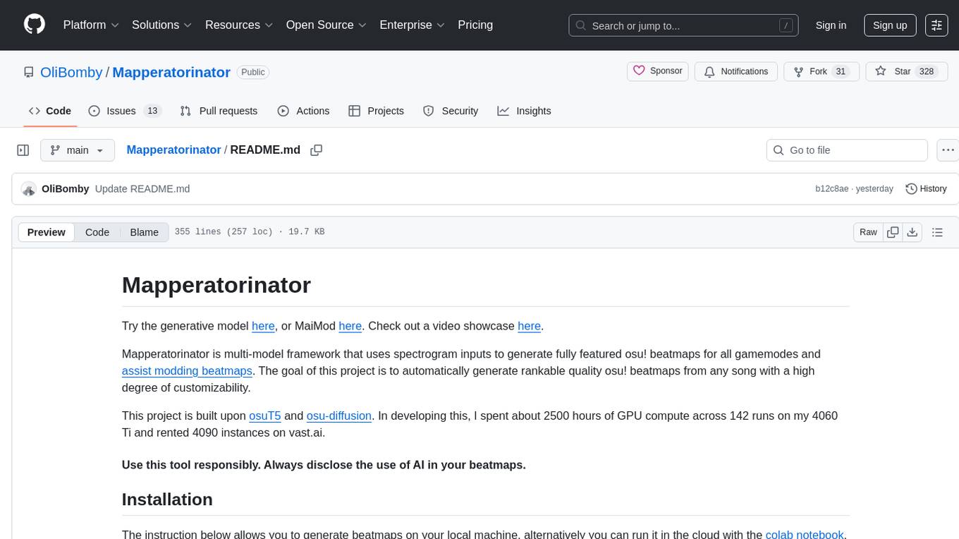
Mapperatorinator is a multi-model framework that uses spectrogram inputs to generate fully featured osu! beatmaps for all gamemodes and assist modding beatmaps. The project aims to automatically generate rankable quality osu! beatmaps from any song with a high degree of customizability. The tool is built upon osuT5 and osu-diffusion, utilizing GPU compute and instances on vast.ai for development. Users can responsibly use AI in their beatmaps with this tool, ensuring disclosure of AI usage. Installation instructions include cloning the repository, creating a virtual environment, and installing dependencies. The tool offers a Web GUI for user-friendly experience and a Command-Line Inference option for advanced configurations. Additionally, an Interactive CLI script is available for terminal-based workflow with guided setup. The tool provides generation tips and features MaiMod, an AI-driven modding tool for osu! beatmaps. Mapperatorinator tokenizes beatmaps, utilizes a model architecture based on HF Transformers Whisper model, and offers multitask training format for conditional generation. The tool ensures seamless long generation, refines coordinates with diffusion, and performs post-processing for improved beatmap quality. Super timing generator enhances timing accuracy, and LoRA fine-tuning allows adaptation to specific styles or gamemodes. The project acknowledges credits and related works in the osu! community.

github

: 327

feedgen

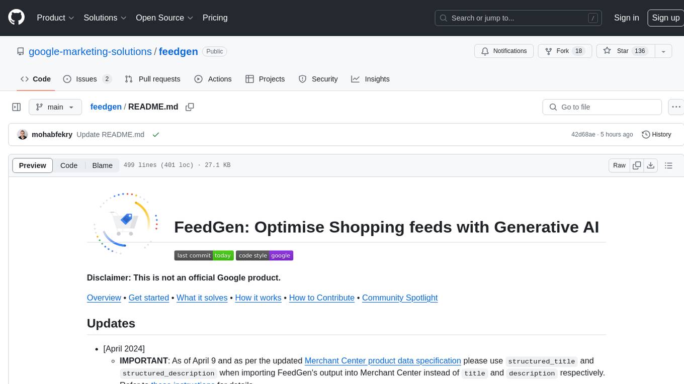
FeedGen is an open-source tool that uses Google Cloud's state-of-the-art Large Language Models (LLMs) to improve product titles, generate more comprehensive descriptions, and fill missing attributes in product feeds. It helps merchants and advertisers surface and fix quality issues in their feeds using Generative AI in a simple and configurable way. The tool relies on GCP's Vertex AI API to provide both zero-shot and few-shot inference capabilities on GCP's foundational LLMs. With few-shot prompting, users can customize the model's responses towards their own data, achieving higher quality and more consistent output. FeedGen is an Apps Script based application that runs as an HTML sidebar in Google Sheets, allowing users to optimize their feeds with ease.

github

: 183

materialize

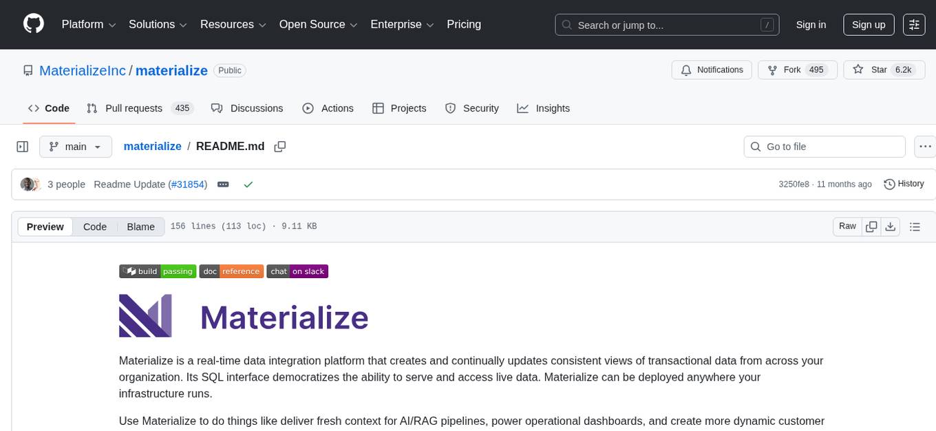
Materialize is a real-time data integration platform that creates and continually updates consistent views of transactional data from across your organization. Its SQL interface democratizes the ability to serve and access live data. Materialize can be deployed anywhere your infrastructure runs. Use Materialize to deliver fresh context for AI/RAG pipelines, power operational dashboards, and create more dynamic customer experiences without building time-consuming custom data pipelines. Materialize focuses on providing correct and consistent answers with minimal latency, and does not ask you to accept either approximate answers or eventual consistency. Materialize answers a query with the correct result on a specific version of your data. Materialize recasts SQL queries as dataflows, which can react efficiently to changes in your data as they happen. Materialize supports a large fraction of PostgreSQL features and is actively expanding support for more built-in PostgreSQL functions. Materialize can read data directly from PostgreSQL or MySQL replication stream, from Kafka, or from SaaS applications via webhooks. Once data is in, define views and perform reads via the PostgreSQL protocol. Materialize supports a comprehensive variety of SQL features, all using the PostgreSQL dialect and protocol. Materialize can incrementally maintain views in the presence of arbitrary inserts, updates, and deletes. Materialize supports recursion that enables incrementally updating tree and graph structures. Materialize is primarily written in Rust.

github

: 6.2k

For similar tasks

chronon

github

: 766

For similar jobs

db2rest

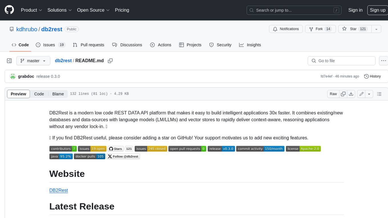
DB2Rest is a modern low-code REST DATA API platform that simplifies the development of intelligent applications. It seamlessly integrates existing and new databases with language models (LMs/LLMs) and vector stores, enabling the rapid delivery of context-aware, reasoning applications without vendor lock-in.

github

: 167

mage-ai

Mage is an open-source data pipeline tool for transforming and integrating data. It offers an easy developer experience, engineering best practices built-in, and data as a first-class citizen. Mage makes it easy to build, preview, and launch data pipelines, and provides observability and scaling capabilities. It supports data integrations, streaming pipelines, and dbt integration.

github

: 7.8k

airbyte

Airbyte is an open-source data integration platform that makes it easy to move data from any source to any destination. With Airbyte, you can build and manage data pipelines without writing any code. Airbyte provides a library of pre-built connectors that make it easy to connect to popular data sources and destinations. You can also create your own connectors using Airbyte's no-code Connector Builder or low-code CDK. Airbyte is used by data engineers and analysts at companies of all sizes to build and manage their data pipelines.

github

: 20.7k

labelbox-python

Labelbox is a data-centric AI platform for enterprises to develop, optimize, and use AI to solve problems and power new products and services. Enterprises use Labelbox to curate data, generate high-quality human feedback data for computer vision and LLMs, evaluate model performance, and automate tasks by combining AI and human-centric workflows. The academic & research community uses Labelbox for cutting-edge AI research.

github

: 135

telemetry-airflow

This repository codifies the Airflow cluster that is deployed at workflow.telemetry.mozilla.org (behind SSO) and commonly referred to as "WTMO" or simply "Airflow". Some links relevant to users and developers of WTMO: * The `dags` directory in this repository contains some custom DAG definitions * Many of the DAGs registered with WTMO don't live in this repository, but are instead generated from ETL task definitions in bigquery-etl * The Data SRE team maintains a WTMO Developer Guide (behind SSO)

github

: 185

airflow

Apache Airflow (or simply Airflow) is a platform to programmatically author, schedule, and monitor workflows. When workflows are defined as code, they become more maintainable, versionable, testable, and collaborative. Use Airflow to author workflows as directed acyclic graphs (DAGs) of tasks. The Airflow scheduler executes your tasks on an array of workers while following the specified dependencies. Rich command line utilities make performing complex surgeries on DAGs a snap. The rich user interface makes it easy to visualize pipelines running in production, monitor progress, and troubleshoot issues when needed.

github

: 44.3k

airbyte-platform

Airbyte is an open-source data integration platform that makes it easy to move data from any source to any destination. With Airbyte, you can build and manage data pipelines without writing any code. Airbyte provides a library of pre-built connectors that make it easy to connect to popular data sources and destinations. You can also create your own connectors using Airbyte's low-code Connector Development Kit (CDK). Airbyte is used by data engineers and analysts at companies of all sizes to move data for a variety of purposes, including data warehousing, data analysis, and machine learning.

github

: 273

chronon

github

: 766