
pycm
Multi-class confusion matrix library in Python
Stars: 1447
PyCM is a Python library for multi-class confusion matrices, providing support for input data vectors and direct matrices. It is a comprehensive tool for post-classification model evaluation, offering a wide range of metrics for predictive models and accurate evaluation of various classifiers. PyCM is designed for data scientists who require diverse metrics for their models.
README:
PyCM is a multi-class confusion matrix library written in Python that supports both input data vectors and direct matrix, and a proper tool for post-classification model evaluation that supports most classes and overall statistics parameters. PyCM is the swiss-army knife of confusion matrices, targeted mainly at data scientists that need a broad array of metrics for predictive models and accurate evaluation of a large variety of classifiers.
| Open Hub |  |
| PyPI Counter | |
| Github Stars |  |
| Branch | master | dev |
| CI |
| Code Quality |
- Check Python Packaging User Guide
- Run
pip install pycm==4.1
- Download Version 4.1 or Latest Source
- Run
pip install .
- Check Conda Managing Package
- Update Conda using
conda update conda - Run
conda install -c sepandhaghighi pycm
- Download and install MATLAB (>=8.5, 64/32 bit)
- Download and install Python3.x (>=3.6, 64/32 bit)
- [x] Select
Add to PATHoption - [x] Select
Install pipoption
- [x] Select
- Run
pip install pycm - Configure Python interpreter
>> pyversion PYTHON_EXECUTABLE_FULL_PATH- Visit MATLAB Examples
>>> from pycm import *
>>> y_actu = [2, 0, 2, 2, 0, 1, 1, 2, 2, 0, 1, 2]
>>> y_pred = [0, 0, 2, 1, 0, 2, 1, 0, 2, 0, 2, 2]
>>> cm = ConfusionMatrix(actual_vector=y_actu, predict_vector=y_pred)
>>> cm.classes
[0, 1, 2]
>>> cm.table
{0: {0: 3, 1: 0, 2: 0}, 1: {0: 0, 1: 1, 2: 2}, 2: {0: 2, 1: 1, 2: 3}}
>>> cm.print_matrix()
Predict 0       1       2
Actual
0       3       0       0

1       0       1       2

2       2       1       3

>>> cm.print_normalized_matrix()
Predict       0             1             2
Actual
0             1.0           0.0           0.0

1             0.0           0.33333       0.66667

2             0.33333       0.16667       0.5

>>> cm.stat(summary=True)
Overall Statistics :

ACC Macro                                                         0.72222
F1 Macro                                                          0.56515
FPR Macro                                                         0.22222
Kappa                                                             0.35484
Overall ACC                                                       0.58333
PPV Macro                                                         0.56667
SOA1(Landis & Koch)                                               Fair
TPR Macro                                                         0.61111
Zero-one Loss                                                     5

Class Statistics :

Classes                                                           0             1             2
ACC(Accuracy)                                                     0.83333       0.75          0.58333
AUC(Area under the ROC curve)                                     0.88889       0.61111       0.58333
AUCI(AUC value interpretation)                                    Very Good     Fair          Poor
F1(F1 score - harmonic mean of precision and sensitivity)         0.75          0.4           0.54545
FN(False negative/miss/type 2 error)                              0             2             3
FP(False positive/type 1 error/false alarm)                       2             1             2
FPR(Fall-out or false positive rate)                              0.22222       0.11111       0.33333
N(Condition negative)                                             9             9             6
P(Condition positive or support)                                  3             3             6
POP(Population)                                                   12            12            12
PPV(Precision or positive predictive value)                       0.6           0.5           0.6
TN(True negative/correct rejection)                               7             8             4
TON(Test outcome negative)                                        7             10            7
TOP(Test outcome positive)                                        5             2             5
TP(True positive/hit)                                             3             1             3
TPR(Sensitivity, recall, hit rate, or true positive rate)         1.0           0.33333       0.5
>>> from pycm import *
>>> cm2 = ConfusionMatrix(matrix={"Class1": {"Class1": 1, "Class2": 2}, "Class2": {"Class1": 0, "Class2": 5}})
>>> cm2
pycm.ConfusionMatrix(classes: ['Class1', 'Class2'])
>>> cm2.classes
['Class1', 'Class2']
>>> cm2.print_matrix()
Predict      Class1       Class2
Actual
Class1       1            2

Class2       0            5

>>> cm2.print_normalized_matrix()
Predict       Class1        Class2
Actual
Class1        0.33333       0.66667

Class2        0.0           1.0

>>> cm2.stat(summary=True)
Overall Statistics :

ACC Macro                                                         0.75
F1 Macro                                                          0.66667
FPR Macro                                                         0.33333
Kappa                                                             0.38462
Overall ACC                                                       0.75
PPV Macro                                                         0.85714
SOA1(Landis & Koch)                                               Fair
TPR Macro                                                         0.66667
Zero-one Loss                                                     2

Class Statistics :

Classes                                                           Class1        Class2
ACC(Accuracy)                                                     0.75          0.75
AUC(Area under the ROC curve)                                     0.66667       0.66667
AUCI(AUC value interpretation)                                    Fair          Fair
F1(F1 score - harmonic mean of precision and sensitivity)         0.5           0.83333
FN(False negative/miss/type 2 error)                              2             0
FP(False positive/type 1 error/false alarm)                       0             2
FPR(Fall-out or false positive rate)                              0.0           0.66667
N(Condition negative)                                             5             3
P(Condition positive or support)                                  3             5
POP(Population)                                                   8             8
PPV(Precision or positive predictive value)                       1.0           0.71429
TN(True negative/correct rejection)                               5             1
TON(Test outcome negative)                                        7             1
TOP(Test outcome positive)                                        1             7
TP(True positive/hit)                                             1             5
TPR(Sensitivity, recall, hit rate, or true positive rate)         0.33333       1.0
-
matrix()andnormalized_matrix()renamed toprint_matrix()andprint_normalized_matrix()inversion 1.5
threshold is added in version 0.9 for real value prediction.
For more information visit Example3
file is added in version 0.9.5 in order to load saved confusion matrix with .obj format generated by save_obj method.
For more information visit Example4
sample_weight is added in version 1.2
For more information visit Example5
transpose is added in version 1.2 in order to transpose input matrix (only in Direct CM mode)
relabel method is added in version 1.5 in order to change ConfusionMatrix classnames.
>>> cm.relabel(mapping={0: "L1", 1: "L2", 2: "L3"})
>>> cm
pycm.ConfusionMatrix(classes: ['L1', 'L2', 'L3'])position method is added in version 2.8 in order to find the indexes of observations in predict_vector which made TP, TN, FP, FN.
>>> cm.position()
{0: {'FN': [], 'FP': [0, 7], 'TP': [1, 4, 9], 'TN': [2, 3, 5, 6, 8, 10, 11]}, 1: {'FN': [5, 10], 'FP': [3], 'TP': [6], 'TN': [0, 1, 2, 4, 7, 8, 9, 11]}, 2: {'FN': [0, 3, 7], 'FP': [5, 10], 'TP': [2, 8, 11], 'TN': [1, 4, 6, 9]}}to_array method is added in version 2.9 in order to returns the confusion matrix in the form of a NumPy array. This can be helpful to apply different operations over the confusion matrix for different purposes such as aggregation, normalization, and combination.
>>> cm.to_array()
array([[3, 0, 0],
       [0, 1, 2],
       [2, 1, 3]])
>>> cm.to_array(normalized=True)
array([[1.     , 0.     , 0.     ],
       [0.     , 0.33333, 0.66667],
       [0.33333, 0.16667, 0.5    ]])
>>> cm.to_array(normalized=True, one_vs_all=True, class_name="L1")
array([[1.     , 0.     ],
[0.22222, 0.77778]])combine method is added in version 3.0 in order to merge two confusion matrices. This option will be useful in mini-batch learning.
>>> cm_combined = cm2.combine(cm3)
>>> cm_combined.print_matrix()
Predict      Class1       Class2
Actual
Class1       2            4

Class2       0            10
plot method is added in version 3.0 in order to plot a confusion matrix using Matplotlib or Seaborn.
>>> cm.plot()>>> from matplotlib import pyplot as plt
>>> cm.plot(cmap=plt.cm.Greens, number_label=True, plot_lib="matplotlib")>>> cm.plot(cmap=plt.cm.Reds, normalized=True, number_label=True, plot_lib="seaborn")ROCCurve, added in version 3.7, is devised to compute the Receiver Operating Characteristic (ROC) or simply ROC curve. In ROC curves, the Y axis represents the True Positive Rate, and the X axis represents the False Positive Rate. Thus, the ideal point is located at the top left of the curve, and a larger area under the curve represents better performance. ROC curve is a graphical representation of binary classifiers' performance. In PyCM, ROCCurve binarizes the output based on the "One vs. Rest" strategy to provide an extension of ROC for multi-class classifiers. Getting the actual labels vector, the target probability estimates of the positive classes, and the list of ordered labels of classes, this method is able to compute and plot TPR-FPR pairs for different discrimination thresholds and compute the area under the ROC curve.
>>> crv = ROCCurve(actual_vector=np.array([1, 1, 2, 2]), probs=np.array([[0.1, 0.9], [0.4, 0.6], [0.35, 0.65], [0.8, 0.2]]), classes=[2, 1])
>>> crv.thresholds
[0.1, 0.2, 0.35, 0.4, 0.6, 0.65, 0.8, 0.9]
>>> auc_trp = crv.area()
>>> auc_trp[1]
0.75
>>> auc_trp[2]
0.75PRCurve, added in version 3.7, is devised to compute the Precision-Recall curve in which the Y axis represents the Precision, and the X axis represents the Recall of a classifier. Thus, the ideal point is located at the top right of the curve, and a larger area under the curve represents better performance. Precision-Recall curve is a graphical representation of binary classifiers' performance. In PyCM, PRCurve binarizes the output based on the "One vs. Rest" strategy to provide an extension of this curve for multi-class classifiers. Getting the actual labels vector, the target probability estimates of the positive classes, and the list of ordered labels of classes, this method is able to compute and plot Precision-Recall pairs for different discrimination thresholds and compute the area under the curve.
>>> crv = PRCurve(actual_vector=np.array([1, 1, 2, 2]), probs=np.array([[0.1, 0.9], [0.4, 0.6], [0.35, 0.65], [0.8, 0.2]]), classes=[2, 1])
>>> crv.thresholds
[0.1, 0.2, 0.35, 0.4, 0.6, 0.65, 0.8, 0.9]
>>> auc_trp = crv.area()
>>> auc_trp[1]
0.29166666666666663
>>> auc_trp[2]
0.29166666666666663This option has been added in version 1.9 to recommend the most related parameters considering the characteristics of the input dataset.
The suggested parameters are selected according to some characteristics of the input such as being balance/imbalance and binary/multi-class.
All suggestions can be categorized into three main groups: imbalanced dataset, binary classification for a balanced dataset, and multi-class classification for a balanced dataset.
The recommendation lists have been gathered according to the respective paper of each parameter and the capabilities which had been claimed by the paper.
>>> cm.imbalance
False
>>> cm.binary
False
>>> cm.recommended_list
['MCC', 'TPR Micro', 'ACC', 'PPV Macro', 'BCD', 'Overall MCC', 'Hamming Loss', 'TPR Macro', 'Zero-one Loss', 'ERR', 'PPV Micro', 'Overall ACC']
is_imbalanced parameter has been added in version 3.3, so the user can indicate whether the concerned dataset is imbalanced or not. As long as the user does not provide any information in this regard, the automatic detection algorithm will be used.
>>> cm = ConfusionMatrix(y_actu, y_pred, is_imbalanced=True)
>>> cm.imbalance
True
>>> cm = ConfusionMatrix(y_actu, y_pred, is_imbalanced=False)
>>> cm.imbalance
FalseIn version 2.0, a method for comparing several confusion matrices is introduced. This option is a combination of several overall and class-based benchmarks. Each of the benchmarks evaluates the performance of the classification algorithm from good to poor and give them a numeric score. The score of good and poor performances are 1 and 0, respectively.
After that, two scores are calculated for each confusion matrices, overall and class-based. The overall score is the average of the score of seven overall benchmarks which are Landis & Koch, Cramer, Matthews, Goodman-Kruskal's Lambda A, Goodman-Kruskal's Lambda B, Krippendorff's Alpha, and Pearson's C. In the same manner, the class-based score is the average of the score of six class-based benchmarks which are Positive Likelihood Ratio Interpretation, Negative Likelihood Ratio Interpretation, Discriminant Power Interpretation, AUC value Interpretation, Matthews Correlation Coefficient Interpretation and Yule's Q Interpretation. It should be noticed that if one of the benchmarks returns none for one of the classes, that benchmarks will be eliminated in total averaging. If the user sets weights for the classes, the averaging over the value of class-based benchmark scores will transform to a weighted average.
If the user sets the value of by_class boolean input True, the best confusion matrix is the one with the maximum class-based score. Otherwise, if a confusion matrix obtains the maximum of both overall and class-based scores, that will be reported as the best confusion matrix, but in any other case, the compared object doesn’t select the best confusion matrix.
>>> cm2 = ConfusionMatrix(matrix={0: {0: 2, 1: 50, 2: 6}, 1: {0: 5, 1: 50, 2: 3}, 2: {0: 1, 1: 7, 2: 50}})
>>> cm3 = ConfusionMatrix(matrix={0: {0: 50, 1: 2, 2: 6}, 1: {0: 50, 1: 5, 2: 3}, 2: {0: 1, 1: 55, 2: 2}})
>>> cp = Compare({"cm2": cm2, "cm3": cm3})
>>> print(cp)
Best : cm2

Rank  Name   Class-Score       Overall-Score
1     cm2    0.50278           0.58095
2     cm3    0.33611           0.52857

>>> cp.best
pycm.ConfusionMatrix(classes: [0, 1, 2])
>>> cp.sorted
['cm2', 'cm3']
>>> cp.best_name
'cm2'From version 4.0, MultiLabelCM has been added to calculate class-wise or sample-wise multilabel confusion matrices. In class-wise mode, confusion matrices are calculated for each class, and in sample-wise mode, they are generated per sample. All generated confusion matrices are binarized with a one-vs-rest transformation.
>>> mlcm = MultiLabelCM(actual_vector=[{"cat", "bird"}, {"dog"}], predict_vector=[{"cat"}, {"dog", "bird"}], classes=["cat", "dog", "bird"])
>>> mlcm.actual_vector_multihot
[[1, 0, 1], [0, 1, 0]]
>>> mlcm.predict_vector_multihot
[[1, 0, 0], [0, 1, 1]]
>>> mlcm.get_cm_by_class("cat").print_matrix()
Predict 0       1
Actual
0       1       0

1       0       1

>>> mlcm.get_cm_by_sample(0).print_matrix()
Predict 0       1
Actual
0       1       0

1       1       1
online_help function is added in version 1.1 in order to open each statistics definition in web browser
>>> from pycm import online_help
>>> online_help("J")
>>> online_help("SOA1(Landis & Koch)")
>>> online_help(2)- List of items are available by calling
online_help()(without argument) - If PyCM website is not available, set
alt_link = True(new inversion 2.4)
PyCM can be used online in interactive Jupyter Notebooks via the Binder or Colab services! Try it out now! :
- Check
ExamplesinDocumentfolder
- Fill an issue and describe it. We'll check it ASAP!
- Please complete the issue template
- Discord : https://discord.com/invite/zqpU2b3J3f
- Website : https://www.pycm.io
- Mailing List : https://mail.python.org/mailman3/lists/pycm.python.org/
- Email : [email protected]
NLnet foundation has supported the PyCM project from version 3.6 to 4.0 through the NGI Assure Fund. This fund is set up by NLnet foundation with funding from the European Commission's Next Generation Internet program, administered by DG Communications Networks, Content, and Technology under grant agreement No 957073.
Python Software Foundation (PSF) grants PyCM library partially for version 3.7. PSF is the organization behind Python. Their mission is to promote, protect, and advance the Python programming language and to support and facilitate the growth of a diverse and international community of Python programmers.
Some parts of the infrastructure for this project are supported by:
If you use PyCM in your research, we would appreciate citations to the following paper :
Haghighi, S., Jasemi, M., Hessabi, S. and Zolanvari, A. (2018). PyCM: Multiclass confusion matrix library in Python. Journal of Open Source Software, 3(25), p.729.
@article{Haghighi2018,
  doi = {10.21105/joss.00729},
  url = {https://doi.org/10.21105/joss.00729},
  year  = {2018},
  month = {may},
  publisher = {The Open Journal},
  volume = {3},
  number = {25},
  pages = {729},
  author = {Sepand Haghighi and Masoomeh Jasemi and Shaahin Hessabi and Alireza Zolanvari},
  title = {{PyCM}: Multiclass confusion matrix library in Python},
  journal = {Journal of Open Source Software}
}
Download PyCM.bib
| JOSS | |
| Zenodo |
Give a ⭐️ if this project helped you!
If you do like our project and we hope that you do, can you please support us? Our project is not and is never going to be working for profit. We need the money just so we can continue doing what we do ;-) .
For Tasks:
Click tags to check more tools for each tasksFor Jobs:
Alternative AI tools for pycm
Similar Open Source Tools

pycm
PyCM is a Python library for multi-class confusion matrices, providing support for input data vectors and direct matrices. It is a comprehensive tool for post-classification model evaluation, offering a wide range of metrics for predictive models and accurate evaluation of various classifiers. PyCM is designed for data scientists who require diverse metrics for their models.
map-anything
MapAnything is an end-to-end trained transformer model for 3D reconstruction tasks, supporting over 12 different tasks including multi-image sfm, multi-view stereo, monocular metric depth estimation, and more. It provides a simple and efficient way to regress the factored metric 3D geometry of a scene from various inputs like images, calibration, poses, or depth. The tool offers flexibility in combining different geometric inputs for enhanced reconstruction results. It includes interactive demos, support for COLMAP & GSplat, data processing for training & benchmarking, and pre-trained models on Hugging Face Hub with different licensing options.
cellseg_models.pytorch
cellseg-models.pytorch is a Python library built upon PyTorch for 2D cell/nuclei instance segmentation models. It provides multi-task encoder-decoder architectures and post-processing methods for segmenting cell/nuclei instances. The library offers high-level API to define segmentation models, open-source datasets for training, flexibility to modify model components, sliding window inference, multi-GPU inference, benchmarking utilities, regularization techniques, and example notebooks for training and finetuning models with different backbones.
Tutel
Tutel MoE is an optimized Mixture-of-Experts implementation that offers a parallel solution with 'No-penalty Parallism/Sparsity/Capacity/Switching' for modern training and inference. It supports Pytorch framework (version >= 1.10) and various GPUs including CUDA and ROCm. The tool enables Full Precision Inference of MoE-based Deepseek R1 671B on AMD MI300. Tutel provides features like all-to-all benchmarking, tensorcore option, NCCL timeout settings, Megablocks solution, and dynamic switchable configurations. Users can run Tutel in distributed mode across multiple GPUs and machines. The tool allows for custom MoE implementations and offers detailed usage examples and reference documentation.

pocketgroq
PocketGroq is a tool that provides advanced functionalities for text generation, web scraping, web search, and AI response evaluation. It includes features like an Autonomous Agent for answering questions, web crawling and scraping capabilities, enhanced web search functionality, and flexible integration with Ollama server. Users can customize the agent's behavior, evaluate responses using AI, and utilize various methods for text generation, conversation management, and Chain of Thought reasoning. The tool offers comprehensive methods for different tasks, such as initializing RAG, error handling, and tool management. PocketGroq is designed to enhance development processes and enable the creation of AI-powered applications with ease.
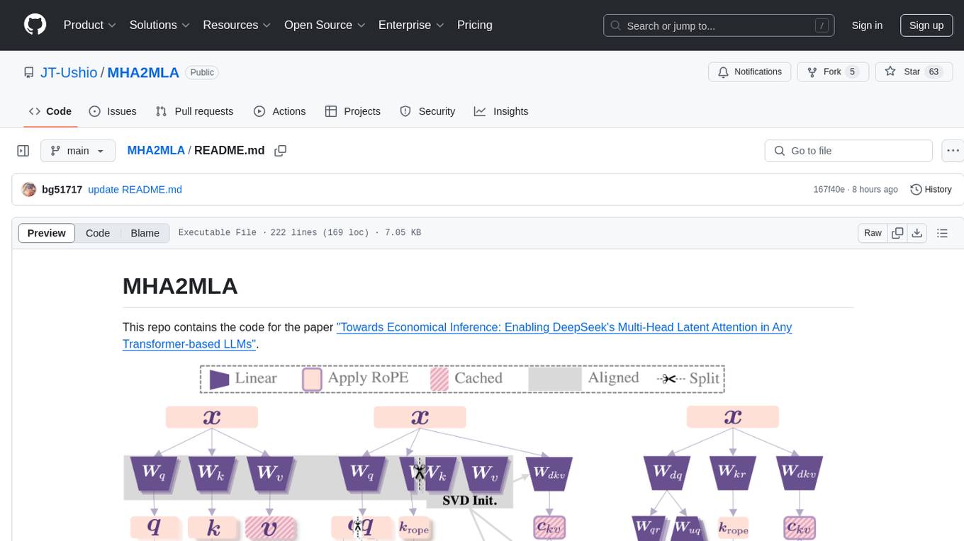
MHA2MLA
This repository contains the code for the paper 'Towards Economical Inference: Enabling DeepSeek's Multi-Head Latent Attention in Any Transformer-based LLMs'. It provides tools for fine-tuning and evaluating Llama models, converting models between different frameworks, processing datasets, and performing specific model training tasks like Partial-RoPE Fine-Tuning and Multiple-Head Latent Attention Fine-Tuning. The repository also includes commands for model evaluation using Lighteval and LongBench, along with necessary environment setup instructions.
serve
Jina-Serve is a framework for building and deploying AI services that communicate via gRPC, HTTP and WebSockets. It provides native support for major ML frameworks and data types, high-performance service design with scaling and dynamic batching, LLM serving with streaming output, built-in Docker integration and Executor Hub, one-click deployment to Jina AI Cloud, and enterprise-ready features with Kubernetes and Docker Compose support. Users can create gRPC-based AI services, build pipelines, scale services locally with replicas, shards, and dynamic batching, deploy to the cloud using Kubernetes, Docker Compose, or JCloud, and enable token-by-token streaming for responsive LLM applications.
client
Gemini PHP is a PHP API client for interacting with the Gemini AI API. It allows users to generate content, chat, count tokens, configure models, embed resources, list models, get model information, troubleshoot timeouts, and test API responses. The client supports various features such as text-only input, text-and-image input, multi-turn conversations, streaming content generation, token counting, model configuration, and embedding techniques. Users can interact with Gemini's API to perform tasks related to natural language generation and text analysis.
dom-to-semantic-markdown
DOM to Semantic Markdown is a tool that converts HTML DOM to Semantic Markdown for use in Large Language Models (LLMs). It maximizes semantic information, token efficiency, and preserves metadata to enhance LLMs' processing capabilities. The tool captures rich web content structure, including semantic tags, image metadata, table structures, and link destinations. It offers customizable conversion options and supports both browser and Node.js environments.
openlrc
Open-Lyrics is a Python library that transcribes voice files using faster-whisper and translates/polishes the resulting text into `.lrc` files in the desired language using LLM, e.g. OpenAI-GPT, Anthropic-Claude. It offers well preprocessed audio to reduce hallucination and context-aware translation to improve translation quality. Users can install the library from PyPI or GitHub and follow the installation steps to set up the environment. The tool supports GUI usage and provides Python code examples for transcription and translation tasks. It also includes features like utilizing context and glossary for translation enhancement, pricing information for different models, and a list of todo tasks for future improvements.

x
Ant Design X is a tool for crafting AI-driven interfaces effortlessly. It is built on the best practices of enterprise-level AI products, offering flexible and diverse atomic components for various AI dialogue scenarios. The tool provides out-of-the-box model integration with inference services compatible with OpenAI standards. It also enables efficient management of conversation data flows, supports rich template options, complete TypeScript support, and advanced theme customization. Ant Design X is designed to enhance development efficiency and deliver exceptional AI interaction experiences.
DB-GPT
DB-GPT is a personal database administrator that can solve database problems by reading documents, using various tools, and writing analysis reports. It is currently undergoing an upgrade. **Features:** * **Online Demo:** * Import documents into the knowledge base * Utilize the knowledge base for well-founded Q&A and diagnosis analysis of abnormal alarms * Send feedbacks to refine the intermediate diagnosis results * Edit the diagnosis result * Browse all historical diagnosis results, used metrics, and detailed diagnosis processes * **Language Support:** * English (default) * Chinese (add "language: zh" in config.yaml) * **New Frontend:** * Knowledgebase + Chat Q&A + Diagnosis + Report Replay * **Extreme Speed Version for localized llms:** * 4-bit quantized LLM (reducing inference time by 1/3) * vllm for fast inference (qwen) * Tiny LLM * **Multi-path extraction of document knowledge:** * Vector database (ChromaDB) * RESTful Search Engine (Elasticsearch) * **Expert prompt generation using document knowledge** * **Upgrade the LLM-based diagnosis mechanism:** * Task Dispatching -> Concurrent Diagnosis -> Cross Review -> Report Generation * Synchronous Concurrency Mechanism during LLM inference * **Support monitoring and optimization tools in multiple levels:** * Monitoring metrics (Prometheus) * Flame graph in code level * Diagnosis knowledge retrieval (dbmind) * Logical query transformations (Calcite) * Index optimization algorithms (for PostgreSQL) * Physical operator hints (for PostgreSQL) * Backup and Point-in-time Recovery (Pigsty) * **Continuously updated papers and experimental reports** This project is constantly evolving with new features. Don't forget to star ⭐ and watch 👀 to stay up to date.
openvino.genai
The GenAI repository contains pipelines that implement image and text generation tasks. The implementation uses OpenVINO capabilities to optimize the pipelines. Each sample covers a family of models and suggests certain modifications to adapt the code to specific needs. It includes the following pipelines: 1. Benchmarking script for large language models 2. Text generation C++ samples that support most popular models like LLaMA 2 3. Stable Diffuison (with LoRA) C++ image generation pipeline 4. Latent Consistency Model (with LoRA) C++ image generation pipeline

educhain
Educhain is a powerful Python package that leverages Generative AI to create engaging and personalized educational content. It enables users to generate multiple-choice questions, create lesson plans, and support various LLM models. Users can export questions to JSON, PDF, and CSV formats, customize prompt templates, and generate questions from text, PDF, URL files, youtube videos, and images. Educhain outperforms traditional methods in content generation speed and quality. It offers advanced configuration options and has a roadmap for future enhancements, including integration with popular Learning Management Systems and a mobile app for content generation on-the-go.
BetaML.jl
The Beta Machine Learning Toolkit is a package containing various algorithms and utilities for implementing machine learning workflows in multiple languages, including Julia, Python, and R. It offers a range of supervised and unsupervised models, data transformers, and assessment tools. The models are implemented entirely in Julia and are not wrappers for third-party models. Users can easily contribute new models or request implementations. The focus is on user-friendliness rather than computational efficiency, making it suitable for educational and research purposes.
CodeTF
CodeTF is a Python transformer-based library for code large language models (Code LLMs) and code intelligence. It provides an interface for training and inferencing on tasks like code summarization, translation, and generation. The library offers utilities for code manipulation across various languages, including easy extraction of code attributes. Using tree-sitter as its core AST parser, CodeTF enables parsing of function names, comments, and variable names. It supports fast model serving, fine-tuning of LLMs, various code intelligence tasks, preprocessed datasets, model evaluation, pretrained and fine-tuned models, and utilities to manipulate source code. CodeTF aims to facilitate the integration of state-of-the-art Code LLMs into real-world applications, ensuring a user-friendly environment for code intelligence tasks.
For similar tasks

pycm
PyCM is a Python library for multi-class confusion matrices, providing support for input data vectors and direct matrices. It is a comprehensive tool for post-classification model evaluation, offering a wide range of metrics for predictive models and accurate evaluation of various classifiers. PyCM is designed for data scientists who require diverse metrics for their models.
instruct-ner
Instruct NER is a solution for complex Named Entity Recognition tasks, including Nested NER, based on modern Large Language Models (LLMs). It provides tools for dataset creation, training, automatic metric calculation, inference, error analysis, and model implementation. Users can create instructions for LLM, build dictionaries with labels, and generate model input templates. The tool supports various entity types and datasets, such as RuDReC, NEREL-BIO, CoNLL-2003, and MultiCoNER II. It offers training scripts for LLMs and metric calculation functions. Instruct NER models like Llama, Mistral, T5, and RWKV are implemented, with HuggingFace models available for adaptation and merging.
InstructGraph
InstructGraph is a framework designed to enhance large language models (LLMs) for graph-centric tasks by utilizing graph instruction tuning and preference alignment. The tool collects and decomposes 29 standard graph datasets into four groups, enabling LLMs to better understand and generate graph data. It introduces a structured format verbalizer to transform graph data into a code-like format, facilitating code understanding and generation. Additionally, it addresses hallucination problems in graph reasoning and generation through direct preference optimization (DPO). The tool aims to bridge the gap between textual LLMs and graph data, offering a comprehensive solution for graph-related tasks.
lighteval
LightEval is a lightweight LLM evaluation suite that Hugging Face has been using internally with the recently released LLM data processing library datatrove and LLM training library nanotron. We're releasing it with the community in the spirit of building in the open. Note that it is still very much early so don't expect 100% stability ^^' In case of problems or question, feel free to open an issue!
Firefly
Firefly is an open-source large model training project that supports pre-training, fine-tuning, and DPO of mainstream large models. It includes models like Llama3, Gemma, Qwen1.5, MiniCPM, Llama, InternLM, Baichuan, ChatGLM, Yi, Deepseek, Qwen, Orion, Ziya, Xverse, Mistral, Mixtral-8x7B, Zephyr, Vicuna, Bloom, etc. The project supports full-parameter training, LoRA, QLoRA efficient training, and various tasks such as pre-training, SFT, and DPO. Suitable for users with limited training resources, QLoRA is recommended for fine-tuning instructions. The project has achieved good results on the Open LLM Leaderboard with QLoRA training process validation. The latest version has significant updates and adaptations for different chat model templates.
Awesome-Text2SQL
Awesome Text2SQL is a curated repository containing tutorials and resources for Large Language Models, Text2SQL, Text2DSL, Text2API, Text2Vis, and more. It provides guidelines on converting natural language questions into structured SQL queries, with a focus on NL2SQL. The repository includes information on various models, datasets, evaluation metrics, fine-tuning methods, libraries, and practice projects related to Text2SQL. It serves as a comprehensive resource for individuals interested in working with Text2SQL and related technologies.
create-million-parameter-llm-from-scratch
The 'create-million-parameter-llm-from-scratch' repository provides a detailed guide on creating a Large Language Model (LLM) with 2.3 million parameters from scratch. The blog replicates the LLaMA approach, incorporating concepts like RMSNorm for pre-normalization, SwiGLU activation function, and Rotary Embeddings. The model is trained on a basic dataset to demonstrate the ease of creating a million-parameter LLM without the need for a high-end GPU.
StableToolBench
StableToolBench is a new benchmark developed to address the instability of Tool Learning benchmarks. It aims to balance stability and reality by introducing features such as a Virtual API System with caching and API simulators, a new set of solvable queries determined by LLMs, and a Stable Evaluation System using GPT-4. The Virtual API Server can be set up either by building from source or using a prebuilt Docker image. Users can test the server using provided scripts and evaluate models with Solvable Pass Rate and Solvable Win Rate metrics. The tool also includes model experiments results comparing different models' performance.
For similar jobs
weave
Weave is a toolkit for developing Generative AI applications, built by Weights & Biases. With Weave, you can log and debug language model inputs, outputs, and traces; build rigorous, apples-to-apples evaluations for language model use cases; and organize all the information generated across the LLM workflow, from experimentation to evaluations to production. Weave aims to bring rigor, best-practices, and composability to the inherently experimental process of developing Generative AI software, without introducing cognitive overhead.

LLMStack
LLMStack is a no-code platform for building generative AI agents, workflows, and chatbots. It allows users to connect their own data, internal tools, and GPT-powered models without any coding experience. LLMStack can be deployed to the cloud or on-premise and can be accessed via HTTP API or triggered from Slack or Discord.

VisionCraft
The VisionCraft API is a free API for using over 100 different AI models. From images to sound.

kaito
Kaito is an operator that automates the AI/ML inference model deployment in a Kubernetes cluster. It manages large model files using container images, avoids tuning deployment parameters to fit GPU hardware by providing preset configurations, auto-provisions GPU nodes based on model requirements, and hosts large model images in the public Microsoft Container Registry (MCR) if the license allows. Using Kaito, the workflow of onboarding large AI inference models in Kubernetes is largely simplified.

PyRIT
PyRIT is an open access automation framework designed to empower security professionals and ML engineers to red team foundation models and their applications. It automates AI Red Teaming tasks to allow operators to focus on more complicated and time-consuming tasks and can also identify security harms such as misuse (e.g., malware generation, jailbreaking), and privacy harms (e.g., identity theft). The goal is to allow researchers to have a baseline of how well their model and entire inference pipeline is doing against different harm categories and to be able to compare that baseline to future iterations of their model. This allows them to have empirical data on how well their model is doing today, and detect any degradation of performance based on future improvements.
tabby
Tabby is a self-hosted AI coding assistant, offering an open-source and on-premises alternative to GitHub Copilot. It boasts several key features: * Self-contained, with no need for a DBMS or cloud service. * OpenAPI interface, easy to integrate with existing infrastructure (e.g Cloud IDE). * Supports consumer-grade GPUs.
spear
SPEAR (Simulator for Photorealistic Embodied AI Research) is a powerful tool for training embodied agents. It features 300 unique virtual indoor environments with 2,566 unique rooms and 17,234 unique objects that can be manipulated individually. Each environment is designed by a professional artist and features detailed geometry, photorealistic materials, and a unique floor plan and object layout. SPEAR is implemented as Unreal Engine assets and provides an OpenAI Gym interface for interacting with the environments via Python.

Magick
Magick is a groundbreaking visual AIDE (Artificial Intelligence Development Environment) for no-code data pipelines and multimodal agents. Magick can connect to other services and comes with nodes and templates well-suited for intelligent agents, chatbots, complex reasoning systems and realistic characters.


